Background

This is Mini-Challenge 3 of VAST Challenge 2023.

FishEye International, a non-profit focused on countering illegal, unreported, and unregulated (IUU) fishing, has been given access to an international finance corporation’s database on fishing related companies. They have transformed the database into a knowledge graph. It includes information about companies, owners, workers, and financial status. FishEye is aiming to use this graph to identify anomalies that could indicate a company is involved in IUU.

Task

Develop a visual analytics process to find similar businesses and group them. This analysis should focus on a business’s most important features and present those features clearly to the user. Limit your response to 400 words and 5 images.

Data preparation

Installing and launching R packages

Show the code

pacman::p_load(jsonlite, tidygraph, ggraph, 
               visNetwork, graphlayouts, ggforce, 
               skimr, tidytext, tidyverse,tm,topicmodels,reshape2,ggplot2,wordcloud,pals,Snowballac,Lda,Ldatuning,kableExtra,DT,flextable,remotes,ldatuning,igraph,qgraph,
               topicmodels.utils,LDAvis,tsne, semnet, servr,devtools)

Import data

Show the code

mc3_data <- fromJSON("data/MC3.json")

Extracting edges

Convert data type from list to character by mutate and as.character

Show the code

mc3_edges <- as_tibble(mc3_data$links) %>% 
  distinct() %>%
  mutate(source = as.character(source),
         target = as.character(target),
         type = as.character(type)) %>%
  group_by(source, target, type) %>%
    summarise(weights = n(),.groups = "drop") %>%
  filter(source!=target)

Extracting nodes

Same country may have different id, so cannot use distinct function, or some ids may be excluded
revenue_omu should be numerical value, so first transform the list into character, then need to transform into numeric
Reorder the dataframe column sequence by select, with id coming first
Replace NA value in revenue_omu with 0
Replace “character[0] in product_services with blank

Show the code

mc3_nodes <- as_tibble(mc3_data$nodes) %>% 
  mutate(country = as.character(country),
         id = as.character(id),
         product_services = as.character(product_services),
         revenue_omu = as.numeric(as.character(revenue_omu)),
         type = as.character(type)) %>% 
  select(id, country, type, revenue_omu, product_services) %>%
mutate(revenue_omu = replace(revenue_omu, is.na(revenue_omu), 0), product_services = replace(product_services, product_services == "character(0)", ""))

Data exploration

Edge dataframe

Display the summary statistics

Show the code

skim(mc3_edges)

Data summary
Name	mc3_edges
Number of rows	24036
Number of columns	4
_______________________
Column type frequency:
character	3
numeric	1
________________________
Group variables	None

Variable type: character

skim_variable	complete_rate	min	max	n_unique
source	1	6	700	12856
target	1	6	28	21265
type	1	16	16	2

Variable type: numeric

skim_variable	n_missing	complete_rate	mean	sd	p0	p25	p50	p75	p100	hist
weights	0	1	1	0	1	1	1	1	1	▁▁▇▁▁

Display interactive table

Show the code

DT::datatable(mc3_edges)

Nodes dataframe

No missing values in mc3_nodes

Show the code

skim(mc3_nodes)

Data summary
Name	mc3_nodes
Number of rows	27622
Number of columns	5
_______________________
Column type frequency:
character	4
numeric	1
________________________
Group variables	None

Variable type: character

skim_variable	complete_rate	min	max	empty	n_unique
id	1	6	64	0	22929
country	1	2	15	0	100
type	1	7	16	0	3
product_services	1	0	1737	18959	3244

Variable type: numeric

skim_variable	n_missing	complete_rate	mean	sd	p0	p25	p50	p75	p100	hist
revenue_omu	0	1	402863.8	8583224	0	0	0	0	310612303	▇▁▁▁▁

Show the code

DT::datatable(mc3_nodes)

Text processing

Perform basic text sensing using tidytext package for product_services in nodes dataframe.

Tokenisation

Split text in product_services field into words with unnest_token() of tidytext.

word: output column name that will be created as the text is unnested into it
product_services: input column that the text comes from
By default, punctuation has been stripped. (Use the to_lower = FALSE argument to turn off this behavior).
By default, unnest_tokens() converts the tokens to lowercase, which makes them easier to compare or combine with other datasets.

Show the code

token_nodes <- mc3_nodes %>% 
  unnest_tokens(word,product_services)

Show the code

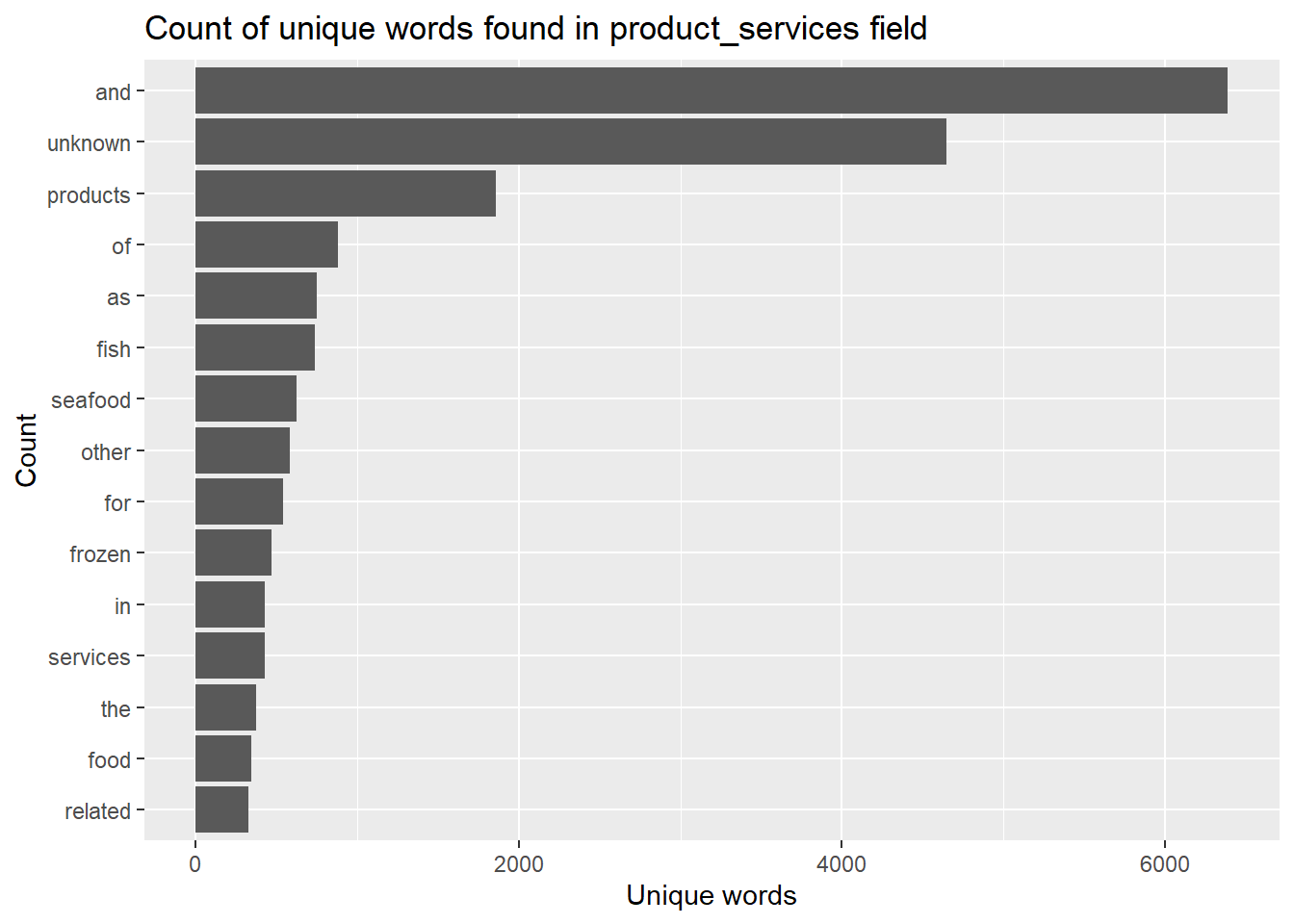
token_nodes %>% 
  count(word,sort =TRUE) %>% 
  top_n(15) %>% 
# reordered according to the values in the n variable
  mutate(word = reorder(word,n)) %>% 
  ggplot(aes(x=word,y=n))+
  geom_col()+xlab(NULL)+
  coord_flip()+
  labs(x = "Count",
      y = "Unique words",
      title = "Count of unique words found in product_services field")

Many of the frequent words are meaningless, such as ‘and’, so need to remove these words.

Removing stop words

Use stop_words in the tidytext package to clean up stop words.

Load the stop_words data included with tidytext.
Then anti_join() of dplyr package is used to remove all stop words from the analysis, only the rows from token_nodesthat do not have a match in stop_words are retained in the result.

Show the code

stopword_removed <- token_nodes %>% 
  anti_join(stop_words)

Show the code

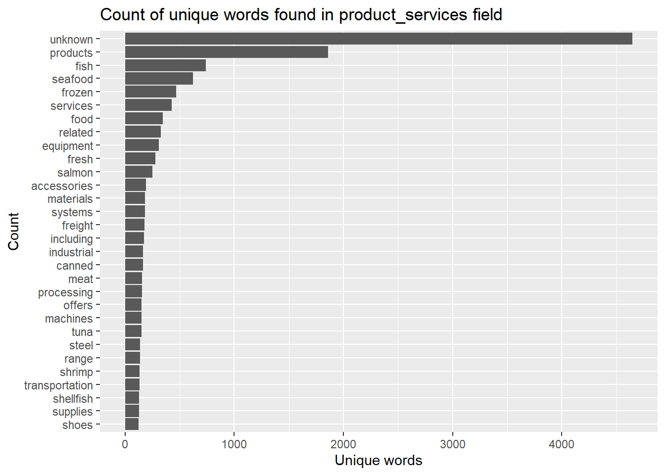
stopword_removed %>% 
  count(word, sort = TRUE) %>% 
  top_n(30) %>% 
  mutate(word = reorder(word,n)) %>% 
  ggplot(aes(x=word,y=n))+
  geom_col()+xlab(NULL)+
  coord_flip()+
  labs(x = "Count",
      y = "Unique words",
      title = "Count of unique words found in product_services field")

There are still some meaningless words, including “unknown, related, including, range”, so extend the stopword dataframe and remove these words.

Show the code

extended_stopwords <- stop_words %>% 
  bind_rows(data.frame(word = c('unknown','related','including','range','products')))

stopword_removed_2 <- token_nodes %>% 
  anti_join(extended_stopwords)

#remove s at the end of each word
stopword_removed_2$word <- gsub("(.*)s$", '\\1', stopword_removed_2$word)

Show the code

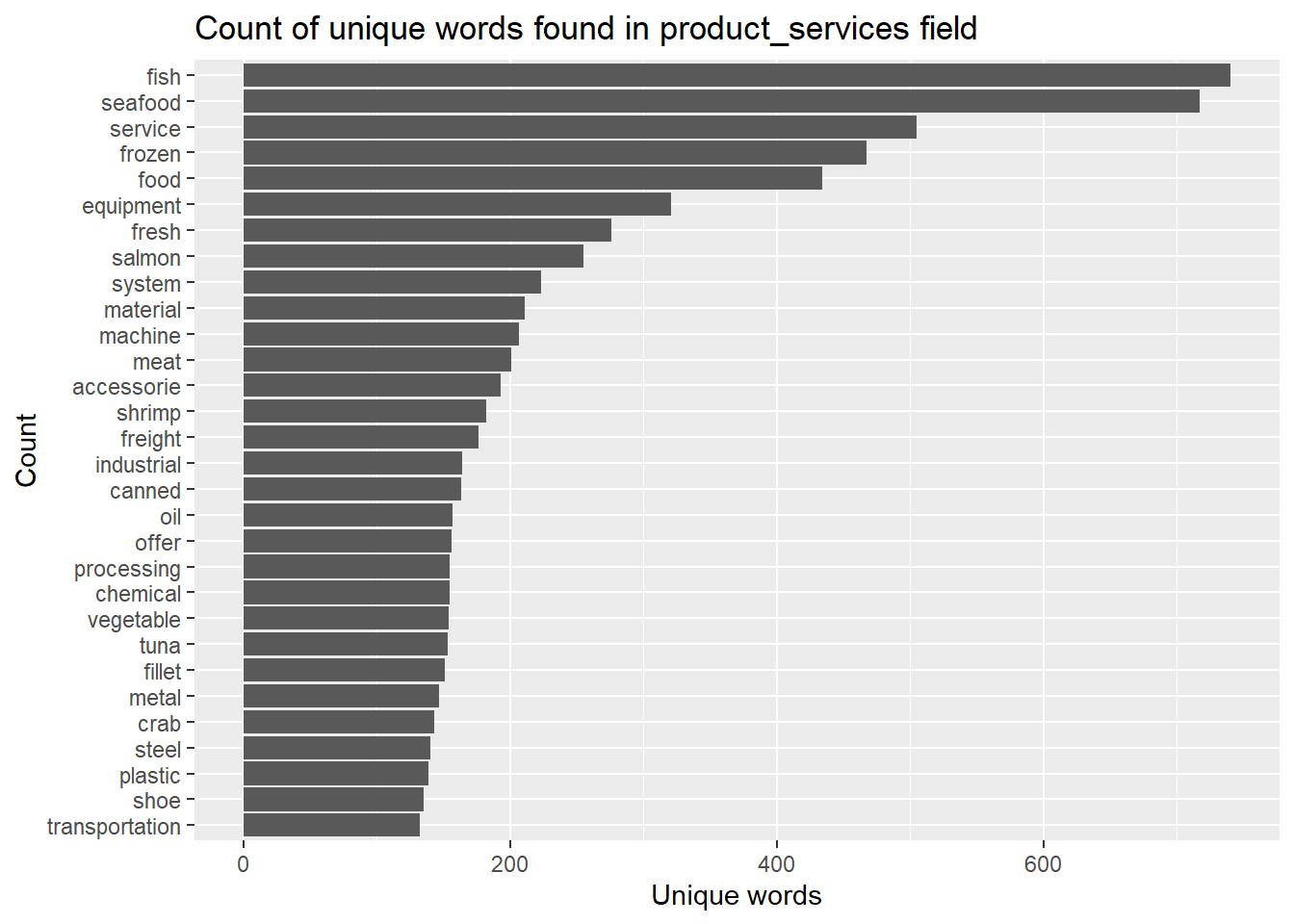
stopword_removed_2 %>% 
  count(word, sort = TRUE) %>% 
  top_n(30) %>% 
  mutate(word = reorder(word,n)) %>% 
  ggplot(aes(x=word,y=n))+
  geom_col()+xlab(NULL)+
  coord_flip()+
  labs(x = "Count",
      y = "Unique words",
      title = "Count of unique words found in product_services field")

Topic modelling

Create a DTM(document term matrix) to capture the frequency of words across dataframe, then filtering terms based on frequency.

Show the code

# compute document term matrix with terms >= minimumFrequency
minimumFrequency <- 5
DTM <- DocumentTermMatrix(stopword_removed_2$word,control = list(bounds =list(global = c(minimumFrequency, Inf))))
dim(DTM)

[1] 43445  1632

Show the code

# exclude empty rows in DTM
row_sums <- slam::row_sums(DTM)>0
DTM <- DTM[row_sums,]

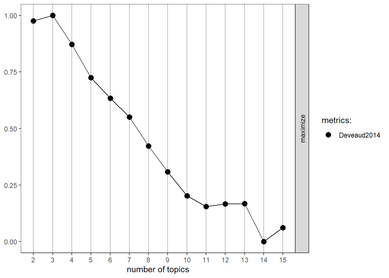
To determine the optimal number of topics, using the “Deveaud2014” metric for topic coherence, select 3 topics that yields a higher value, indicating a stronger degree of similarity between words within each topic.

Show the code

result <- ldatuning::FindTopicsNumber(
  DTM,
  topics = seq(from = 2, to = 15, by =1),
  metrics = "Deveaud2014",
  method = 'Gibbs',
  control = list(seed = 1234),
  verbose = TRUE
)

fit models... done.
calculate metrics:
  Deveaud2014... done.

Show the code

FindTopicsNumber_plot(result)

Build topic model with number of four, with ‘Gibbs’ sampling method, and with verbose = 100 to display the details of iteration progress.

Show the code

k <- 3
set.seed(1234)
topicmodel <- LDA(DTM,k,method = 'Gibbs',control = list(iter = 500, verbose = 100))

K = 3; V = 1632; M = 35285
Sampling 500 iterations!
Iteration 100 ...
Iteration 200 ...
Iteration 300 ...
Iteration 400 ...
Iteration 500 ...
Gibbs sampling completed!

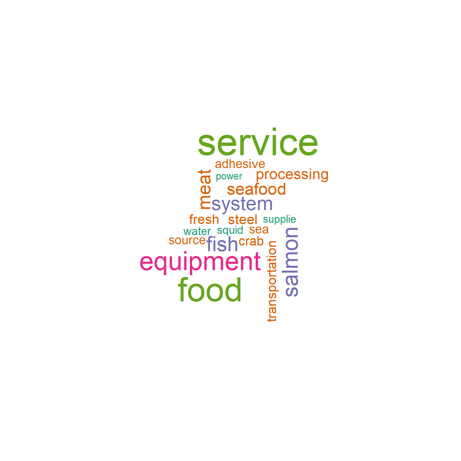
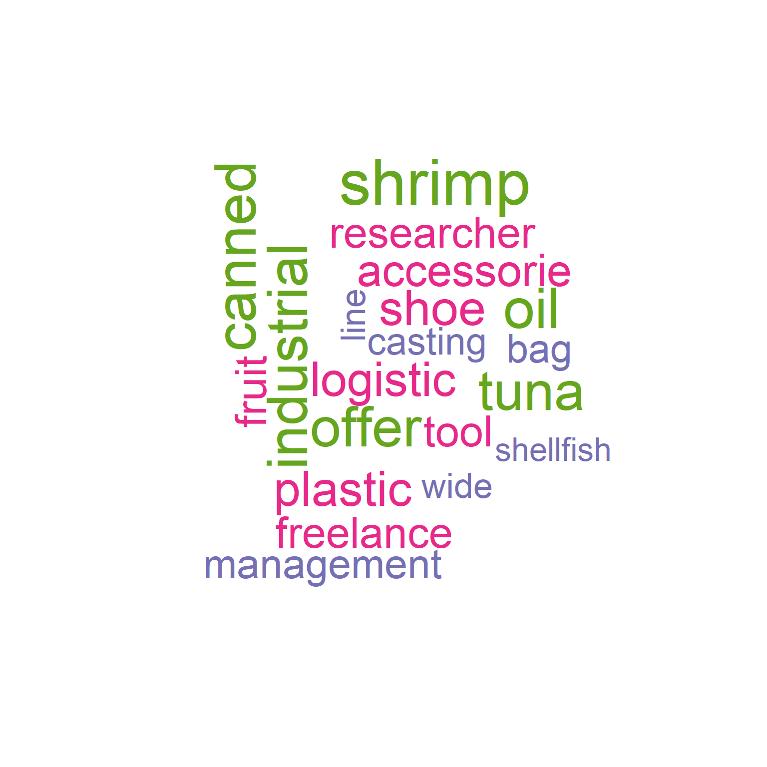
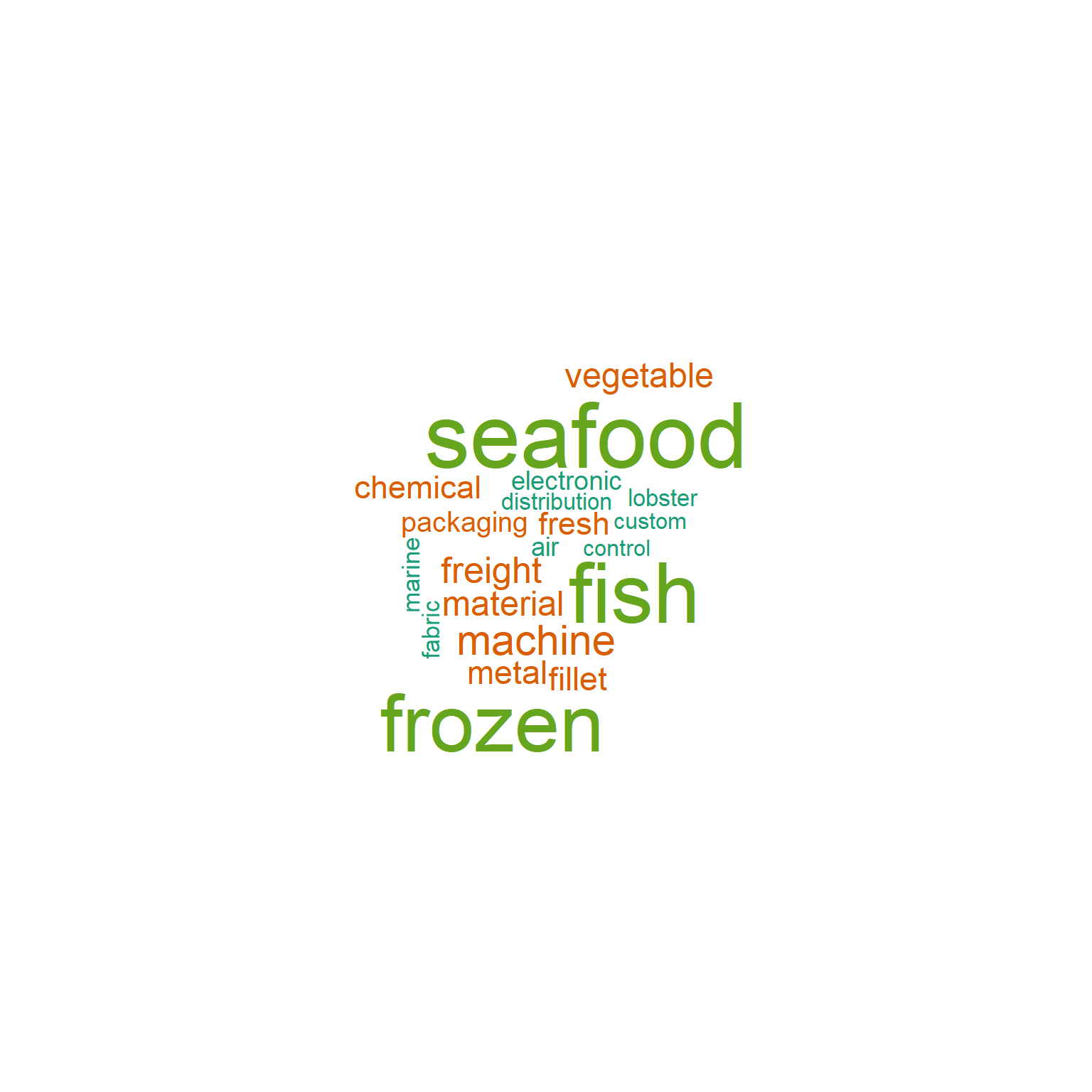
From the word cloud and feature bar plot, we can see the important features within similar company group.

Show the code

# see the probability of each word belonging to each topic
topicmodel_tidy <- tidy(topicmodel,matrix ='beta')

top_terms <- topicmodel_tidy %>%
  group_by(topic) %>%
  top_n(20, beta) %>%
  arrange(topic, desc(beta))

# Create a separate word cloud for each topic

for (i in 1:3) {
  topic_words <- subset(top_terms, topic == i)
  wordcloud(
    words = topic_words$term,
    freq = topic_words$beta,
    colors = brewer.pal(5, 'Dark2')
  )
}

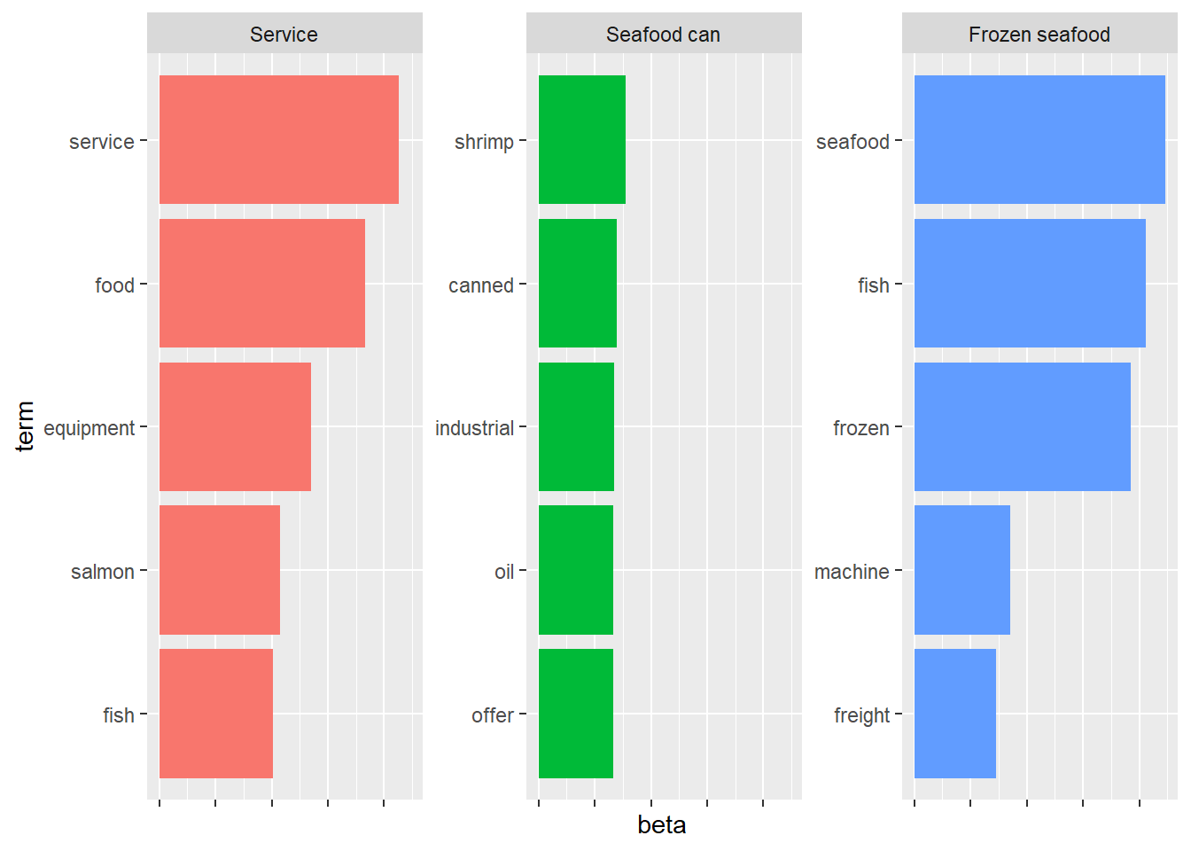
Based on the top feature, categorizing the groups of companies into the company type shown as below.

Show the code

# see the probability of each word belonging to each topic
topicmodel_tidy <- tidy(topicmodel,matrix ='beta')

# find top 5 words with maximum probability in each topic
top_terms <- topicmodel_tidy %>% 
  group_by(topic) %>% 
  slice_max(beta, n = 5) %>% 
  arrange(topic, -beta)

# visulize by ggplot
top_terms %>% 
  mutate(term = reorder_within(term,beta,topic)) %>% 
  ggplot(aes(beta, term, fill = factor(topic)))+
  geom_col(show.legend = FALSE)+
  facet_wrap(~topic, scales = "free_y",labeller = labeller(topic = c("1" = "Service", "2" = "Seafood can", "3" = "Frozen seafood"))
             )+
  scale_y_reordered()+
  theme(axis.text.x = element_blank())

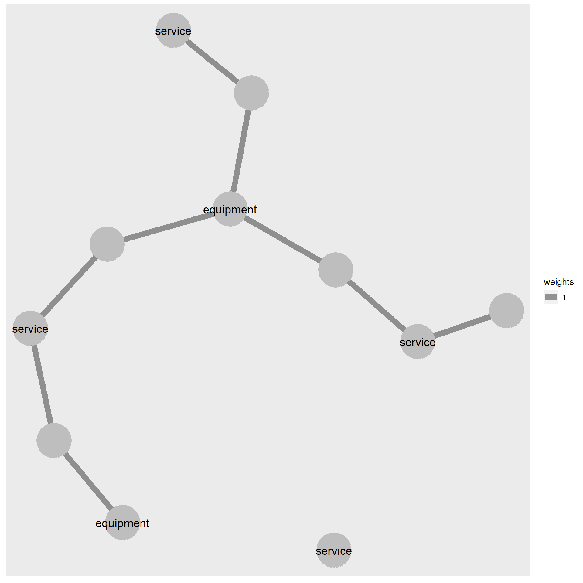
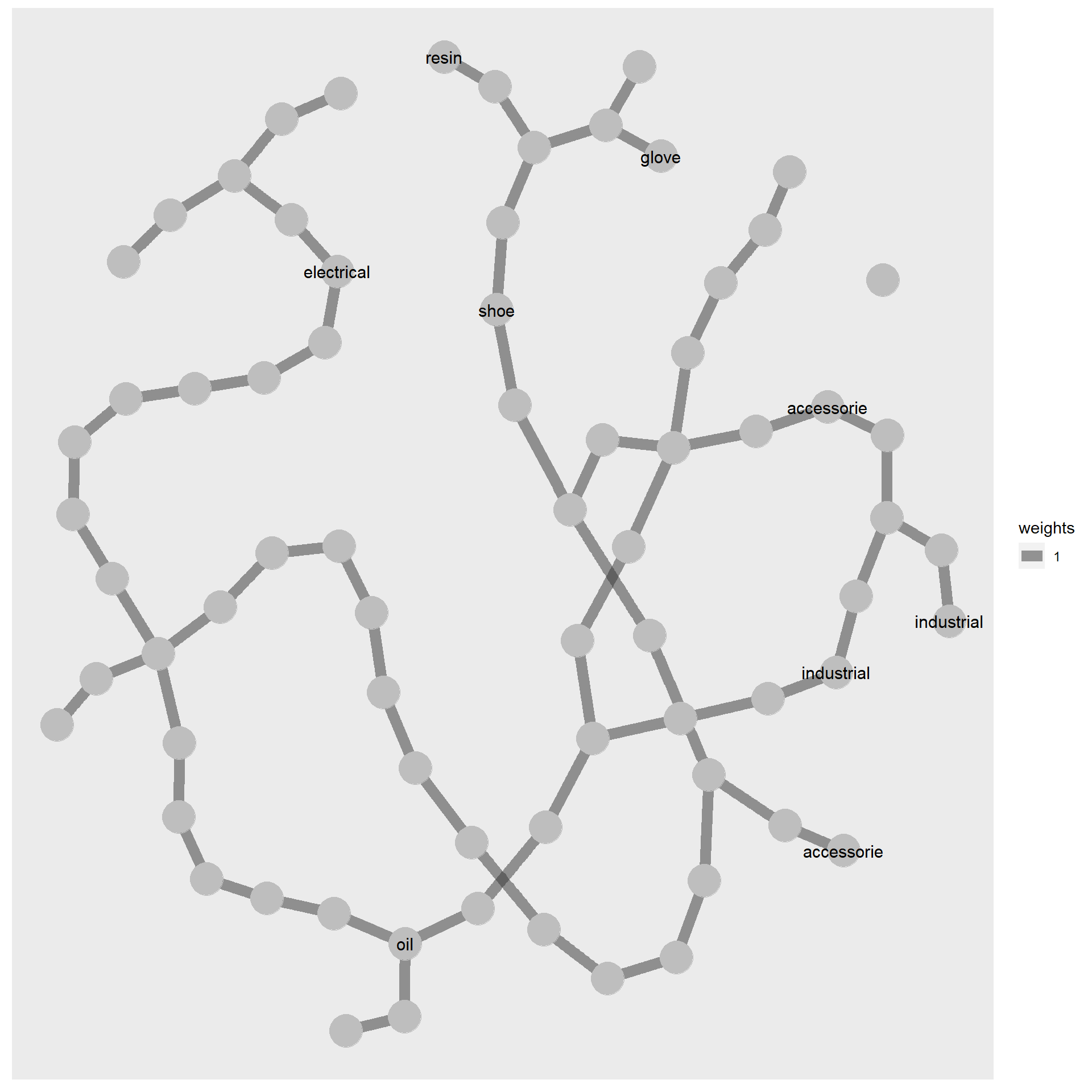
Network visual

Build tidygraph

Derive the highest beta for each term in topic modelling dataframe

Show the code

topicmodel <- topicmodel_tidy %>% 
  group_by(term) %>% 
   slice(which.max(beta)) %>%
  ungroup()

Join topic model result with node

Show the code

mc3_nodes_update <- left_join(stopword_removed_2, topicmodel, by = c("word"= "term"))

mc3_nodes_update <- na.omit(mc3_nodes_update)

Selecting the word with the highest beta value for each company

Show the code

mc3_nodes_topic <- mc3_nodes_update %>%
  group_by(id, country, type, revenue_omu) %>%
  slice(which.max(beta)) %>%
  ungroup() %>% 
  distinct()

Topic 1

Show the code

mc3_nodes_topic1 <- mc3_nodes_topic %>% 
  filter(topic ==1)

MC3_edge <- mc3_edges %>% 
  filter(source %in% mc3_nodes_topic1$id | target %in% mc3_nodes_topic1$id) %>% 
  rename(from = source) %>%
  rename(to = target) 

id1 <- MC3_edge %>%
  select(from) %>%
  rename(id = from)
id2 <- MC3_edge %>%
  select(to) %>%
  rename(id = to)

mc3_node <- rbind(id1, id2) %>%
  distinct() %>% 
  left_join(mc3_nodes_topic1, by = 'id')

MC3_graph <- tbl_graph(nodes = mc3_node,
                       edges = MC3_edge,
                       directed =FALSE)%>%
  mutate(betweenness_centrality = centrality_betweenness())

If filter by high betweenness centrality, can see that company features are equipment and service only.

Show the code

MC3_graph %>%
  filter(betweenness_centrality >= 2000) %>%
ggraph(layout = "fr")+
  geom_edge_link(aes(width = weights), alpha = 0.50, edge_color = "grey20") +
  geom_node_point(color = "gray", size = 20, show.legend = FALSE) +
  geom_node_text(aes(label = word),  colour = 'black', size=5,show.legend = FALSE)

Topic 2

Show the code

mc3_nodes_topic2 <- mc3_nodes_topic %>% 
  filter(topic ==2)

MC3_edge <- mc3_edges %>% 
  filter(source %in% mc3_nodes_topic$id | target %in% mc3_nodes_topic1$id) %>% 
  rename(from = source) %>%
  rename(to = target) 

id1 <- MC3_edge %>%
  select(from) %>%
  rename(id = from)
id2 <- MC3_edge %>%
  select(to) %>%
  rename(id = to)

mc3_node <- rbind(id1, id2) %>%
  distinct() %>% 
  left_join(mc3_nodes_topic2, by = 'id')

MC3_graph <- tbl_graph(nodes = mc3_node,
                       edges = MC3_edge,
                       directed =FALSE)%>%
  mutate(betweenness_centrality = centrality_betweenness(),
         closeness_centrality = centrality_closeness())

We can see that some company features with high betweenness centrality look abnormal, including unrelated features to fishing such as shoe and glove.

Show the code

MC3_graph %>%
  filter(betweenness_centrality >= 100000) %>%
ggraph(layout = "fr")+
  geom_edge_link(aes(width = weights), alpha = 0.50, edge_color = "grey20") +
  geom_node_point(color = "gray", size = 10, show.legend = FALSE) +
  geom_node_text(aes(label = word),  colour = 'black', size=4,show.legend = FALSE)

Topic 3

Show the code

mc3_nodes_topic3 <- mc3_nodes_topic %>% 
  filter(topic ==3)

MC3_edge <- mc3_edges %>% 
  filter(source %in% mc3_nodes_topic3$id | target %in% mc3_nodes_topic1$id) %>% 
  rename(from = source) %>%
  rename(to = target) 

id1 <- MC3_edge %>%
  select(from) %>%
  rename(id = from)
id2 <- MC3_edge %>%
  select(to) %>%
  rename(id = to)

mc3_node <- rbind(id1, id2) %>%
  distinct() %>% 
  left_join(mc3_nodes_topic3, by = 'id')

MC3_graph <- tbl_graph(nodes = mc3_node,
                       edges = MC3_edge,
                       directed =FALSE)%>%
  mutate(betweenness_centrality = centrality_betweenness(),
         closeness_centrality = centrality_closeness())

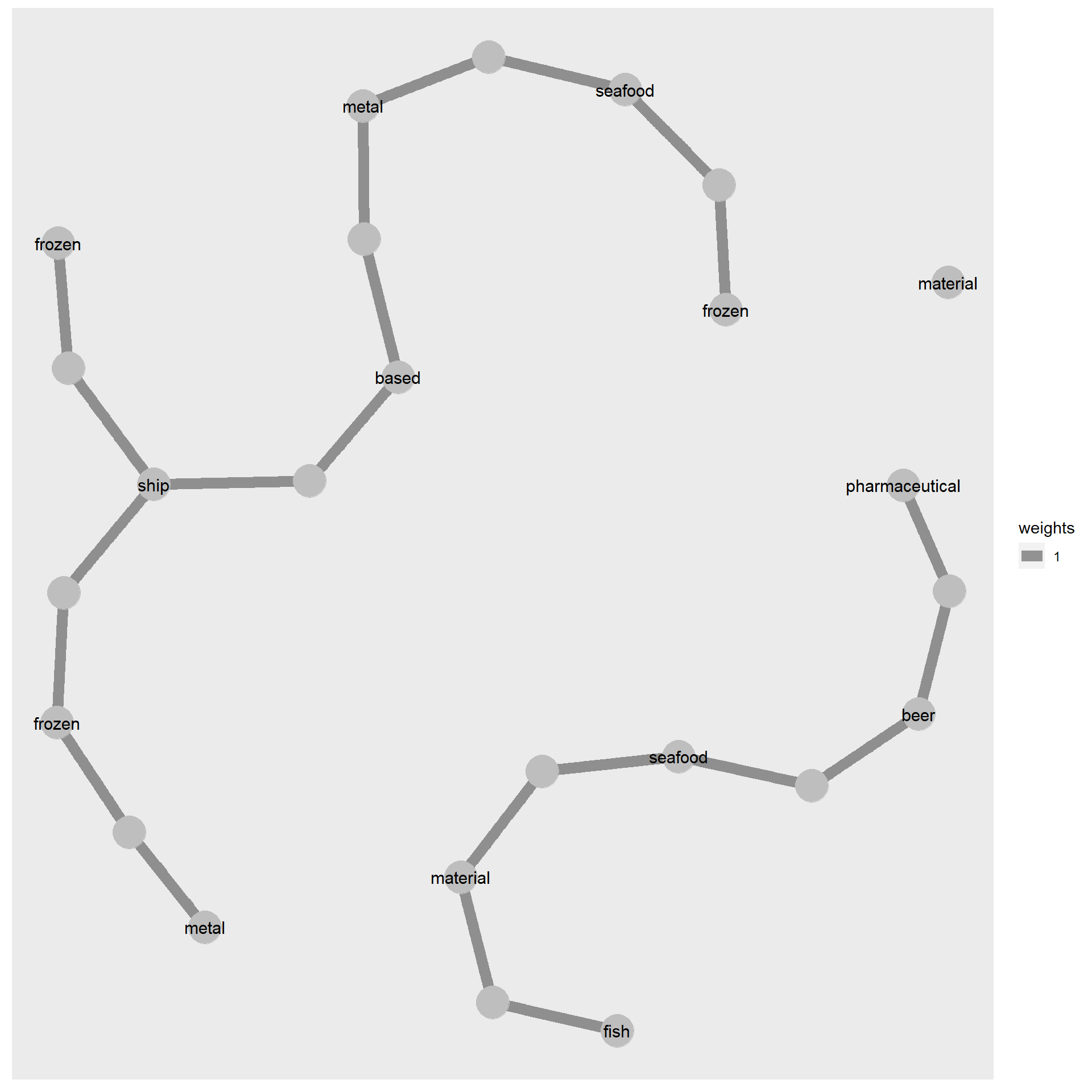
For nodes with high betweenness centrality in topic 3, it is expected to see a majority of them being related to frozen/seafood and fish. However, there are some companies with unrelated features such as pharmaceutical and metal that have unexpectedly high betweenness centrality.

Show the code

MC3_graph %>%
  filter(betweenness_centrality >= 5000) %>%
ggraph(layout = "fr")+
  geom_edge_link(aes(width = weights), alpha = 0.50, edge_color = "grey20") +
  geom_node_point(color = "gray", size = 10, show.legend = FALSE) +
  geom_node_text(aes(label = word),  colour = 'black', size=4,show.legend = FALSE)